Reproducible Research in High-Throughput Biology: A Case Study
Paolo Sonego
November 30th, 2012
Overview
- What is Reproducible Research?
- Why is Reproducible Research important in Scientific Research?
- Tools for Reproducible Research and Literate Programming
- Reproducible Research in the Analysis of High-Throughput Biological Data.
- A Case Study
Introduction
- Reproducibility in Science
- Reproducible Research
- Literate Programming
What is Reproducible Research?
- Reproducible research allows the reader of the article to replicate the entire analysis on his own.
- It use the Literate Programming paradigm (invented by Donald Knuth) to combine the input data, the source code, the literate description of the adopted procedures and the results (tables, plots, etc.) in a unique document both producing and depicting the analysis.
- As a rule of thumb, we have an article following the Reproducible Research paradigm if the author provide the reader with all the information required for replicating the analysis:
- it provides the original (raw) data
- methods and algorithms are properly and fully described
- methods can be reproduced
- the analysis can be extended to independent datasets
Why Reproducible Research is so important?
- omics studies are spreading the basis for new clinical trials and treatment decisions
- Make your life easier in data analysis daily practice
The Anil Potti Story
- “Genomic Signatures to Guide the Use of Chemotherapeutics”, Potti et al (2006), Nature Medicine, 12:1294-1300.
- The main conclusion of the paper is that we can use microarray data from cell lines to define drug response signatures, which can be used to predict whether patients will respond.
- Keith Baggerly and Kevin Coombes Bioinformatic Statisticians at MD Anderson Cancer Center contacted Anil Potti to get hold of the source code for the analysis without success.
The two bioinformaticians employed forensic bioinformatics in order to recreate the data by matching public sources to measurements from the printed graphs, and figured out that there were gross data errors in the article: labels transposed, data duplicated, etc. . The conclusions were completely bunk…
- All the performed analysis by Baggerly and Coombes were conducted following a state of art Reproducible Research approach (see here) and depicted in “Deriving Chemosensitivity from Cell Lines: Forensic Bioinformatics and Reproducible Research in High-Throughput Biology” by Keith A. Baggerly and Kevin R. Coombes, Annals of Applied Statistics, 2009 3(4):1309-1334.
Further more the two bioinformaticians collected all sort of documents, talk, video about the subject and make them available from this link.
The Anil Potti Story - Conclusion
- Ten high-impact research papers authored by Potti were retracted.
- The American Cancer Society stopped payment of a five-year-grant to Potti
and Duke University was forced to reimbursed the American Cancer Society for the grant.
- Three clinical trials at Duke University Medical Center based on Potti’s research were stopped.
Reproducible Research in daily practice
- “We have performed some new experiments, can you add them and re-run the analysis you performed X months ago?”
- “Our previous analyst left, can you re-analyze my data with the same methods he used and produce a comprehensible report?”
- “Can you write the methods section for an article based on the analysis you made as service 1 year ago?”
- A programming language for use in typesetting designed from scratch by Donald Knuth in 1970 for his book The Art of Computer Programming.
- TeX is about format, for document designers, LaTeX is all about content, for document writers.
- In other words, the idea behind LaTeX is to shift the focus from the format to the content of your document.
- Pros:
- Very well established and robust
- rich collection of packages (CTAN)
- perfect for research paper, books, thesis, etc.
- well documented
- Cons:
- steep learning curve
- layout is not always a piece of cake
- debugging can be a pain in the …
LaTeX “Hello World”
\documentclass{article}
\title{Hello World}
\author{Paolo Sonego}
\date{November 2012}
\begin{document}
   \maketitle
   Hello world!
\end{document}
Sweave
The de facto standard for Reproducible Research in the R environment.
- Pros:
- embedded in every R-base distribution
- Vignettes (documents depicting packages functionalities) are produced using Sweave (code available)
- quite robust
- Cons:
- stagnant development
- poor documentation and resources compared to alternatives
Sweave “Hello World”
Take a LaTex source file.
Change the file extension from .tex to .Rnw.
Insert a chunk of R code you want to execute between << >>= and a @ sign followed by a space:
<<hello sweave >>=
print(rnorm(50))
@
##  [1] -1.02809  0.58519  0.47856 -1.15948  0.35598 -0.19351 -1.13424  0.63789
##  [9]  1.69889 -1.11168  1.01274 -1.86981 -0.03253 -1.23849  0.65434  0.51970
## [17] -0.17844  0.15562 -0.31640  0.73339  1.58082  0.28131 -0.49190 -0.53323
## [25] -0.64260  0.06578 -1.07761  0.88227 -0.33908 -0.29489  0.65853  0.49415
## [33]  0.91659 -0.20477 -0.33838  1.67765 -0.70644 -0.55799 -0.26238 -0.19877
## [41] -0.49096 -1.33861 -0.39981  0.41306  0.01421 -0.53587  0.48340  2.28866
## [49] -1.33952 -1.84252
Run Sweave to produce Tex, and Stangle to extract the R code
R CMD Sweave helloworld.Rnw
R CMD Stangle helloworld.Rnw
pdflatex helloworld
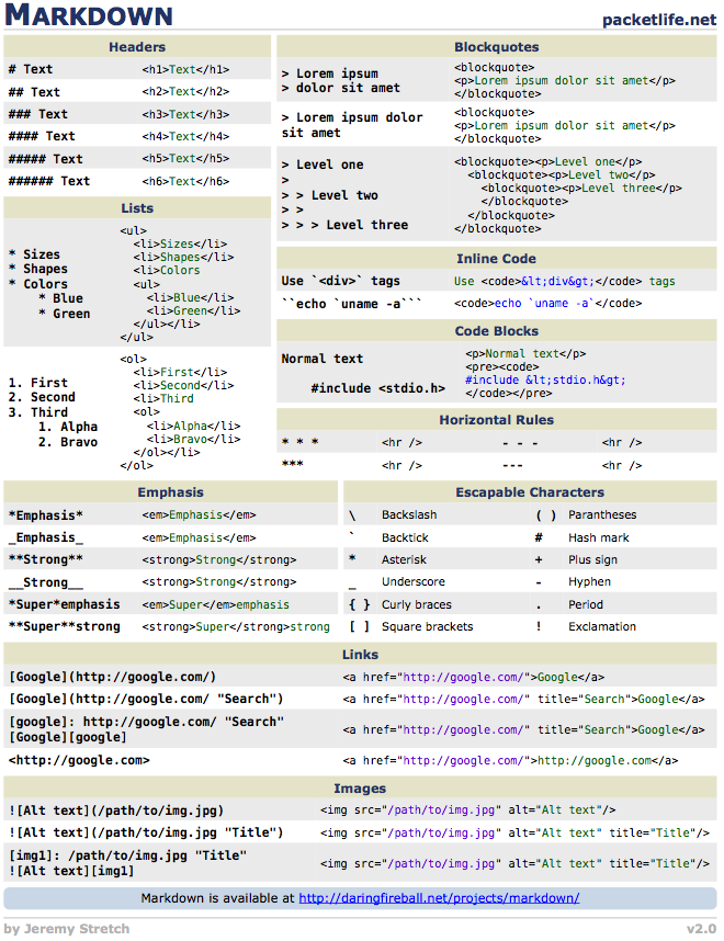
Markdown
- Pros:
- you can learn it in few minutes
- you can produce slides, reports, interactive documents in no time
- quickly spreading
- Cons:
- useful to produce simple documents quickly, not so good with complicated documents such as research paper, books, thesis, etc.
- still in development
- no CTAN
R Markdown
It allows the insertion of R chunks in a markdown file as well as Sweave allows it in a LaTeX file.
```{r hello_rmarkdown}
print(rnorm(50))
```
##  [1]  0.47135  0.33137  1.12405 -1.93464  0.49882 -0.40663  1.70079  1.95296
##  [9]  0.28356  0.46559 -1.60801 -0.51435 -1.14396  1.38524  1.41066 -0.51923
## [17]  0.01728 -1.15363  1.05206 -1.38199 -0.47508  1.18964 -0.35563 -0.41657
## [25] -0.70746  1.41704 -0.65796 -0.11216  0.67053 -0.11592  0.49551 -0.17050
## [33]  0.36816  0.06961 -0.32033 -0.60880 -0.72954 -0.60811 -0.02811  1.25004
## [41] -0.35045  1.64920  1.58694 -0.05738  0.68935 -0.03911  0.94360  1.18036
## [49]  0.45375 -0.04956
- It requires the knitr package for producing a markdown document which can be converted into html, pdf, etc.
knitr
- An R package and powerful tool for extending Sweave features:
- It allows the use of different markup languages: LaTex, Markdown
- Great output with default settings
- Pros:
- good default settings
- out-of-the-box caching system that evaluate chached chunks only when necessary
- great ever-growing documentation and collection of examples (see knitr demo)
- actively developed
- Cons:
- not included in default R distribution
- markdown integration can be better
- not as robust as Sweave
pandoc
Swiss-army knife for converting a markup document in different formats, few examples:
- A pdf file:
pandoc -s report.md -t latex -o report.pdf
- A html file:
pandoc -s report.md -o report.html
- LibreOffice:
pandoc report.md -o report.odt
- Word docx:
pandoc report.md -o report.docx
Versioning and Version Control Systems
- What is Versioning?
- It is the the process of tracking changes of documents by assigning unique ids (strings or numbers) at different unique stages
- What is Revision Control?
- A central place to store your code:
- Backup and recovery
- A recorded history of code changes
- Facilitates collaboration among development team members
- Easy to check out prior code, undo changes, version products
- Why I should use a Revision Control?
- Collaborate on the same project
- Access to different revision of your code
- Save your day!
“Enterprise-class centralized version control for the masses”
Subversion exists to be universally recognized and adopted as an open-source, centralized version control system characterized by its reliability as a safe haven for valuable data; the simplicity of its model and usage; and its ability to support the needs of a wide variety of users and projects, from individuals to large-scale enterprise operations.
svn “Hello World”
svnadmin create SVNrep
mkdir test
touch test/test.txt
svn import test file:///Users/paolo/SVNrep/test ‐m 'Initial import'
rm –r test
svn checkout file:///Users/paolo/SVNrep/test
echo 'Hello World' > test.txt
svn status
svn commit test.txt ‐m'test modified'
svn update
svn diff ‐r 1
git
- Initially developed by Linus Torvalds for Linux kernel development
- fast
- Social features
- Highly adopted in the R Community
Reproducible Research in High-Throughput Biology
- A common generic workflow in Bioinformatics:
- get the data
- download the annotations for your data from on-line resources: Ensembl, USCS Genome Browser, etc.
- download and compile the tools for the analysis
- parse the outputs of the different software using custom code written in X different programming languages
- Feed the intermediate results to other on-line web services: Reactome, DAVID, etc.
- What is wrong?
- web resources can be unstable
- bioinformaticians have to store locally the data and software tailored to the particular analysis
- using different paradigms for the analysis (some times is the only choice) is error prone
R and Bioconductor
Bioconductor
- Bioconductor is an open source project to provide tools for the analysis and comprehension of high-throughput genomic data, based primarily on the R programming language.
- The broad goals of the Bioconductor project are:
- To provide widespread access to a broad range of powerful statistical and graphical methods for the analysis of genomic data.
- To facilitate the inclusion of biological metadata in the analysis of genomic data, e.g. literature data from PubMed, annotation data from Entrez genes.
- To provide a common software platform that enables the rapid development and deployment of extensible, scalable, and interoperable software.
- To further scientific understanding by producing high-quality documentation and reproducible research.
- To train researchers on computational and statistical methods for the analysis of genomic data.
Why Bioconductor is the way to follow for Reproducible Research
- Same programming environment with tools operating and cooperating between them in coherent ways
- easy way to organize projects and create pipelines
- Reproducible Research through Literate Programming out-of-the-box
- Bioconductor repository stores all the past versions of analytical and annotation packages
- For example:
- analysis with Human RNA-Seq data or Affymetrix Human Genome U133 Plus 2.0 Array
- download/install/load the transcript annotation data for RNA-seq
library("TxDb.Hsapiens.UCSC.hg19.knownGene")
or for the specific Affymetrix chip library('hgu133plus2.db')
- use
sessionInfo() to record the state of all my packages and my session
- Later (months, years), you need to repeat the analysis:
- get the recorded
sessionInfo() for the original analysis
- get the original R-version and bioconductor packages from the repositories
- reproduce the analysis
Summary
- Use a Version Control System for recording your source code changes
- Create pipelines producing documents including both the analysis and the working code (Literate Programming)
- Use Bioconductor and include the version of your packages and the session info in the document
- One more thing:
- The Bioconductor team has developed an Amazon Machine Image (AMI) that is optimized for running Bioconductor in the Amazon Elastic Compute Cloud (or EC2) for sequencing tasks.
- storing data, code, packages in a frozen Virtual Machine allows the complete reproducibility of your analysis and make easy to share the results
Case Study
“Reversal of gene expression changes in the colorectal normal-adenoma pathway by NS398 selective COX2 inhibitor, O Galamb et al., British Journal of Cancer (2010) 102, 765–773”
- Aim of the paper:
The aims of this study were to analyse the gene expression modulating effect of NS398 selective COX2 inhibitor on the HT29 colon adenocarcinoma cell line and to correlate this effect to the modulation in gene expression observed during normal-adenoma and normal-CRC transition when biopsy samples were analysed.
- Aim of the our analysis:
- Showing a basic workflow for the analysis of high-throughput data which follows the Reproducible Research approach.
- Verifying whether, following the materials and methods depicted in the manuscript, we were capable of reproduce some of the analysis depicted in the manuscript or not.
Case Study - Conclusion
- We selected to replicate the Class Prediction analysis depicted in the manuscript: The authors taking advantage of the nearest shrunken centroid method (PAM) wanted to identify the gene expressions patterns (signatures) of the contrasts adenoma vs normal biopsy samples and colorectal cancer (CRC) vs normal biopsy samples.
- The results of our analysis were different from the manuscript (they matched them only partially).
- Why this analysis can be replicated exactly?
- No source code for the analyses was included;
- The versions of the different packages were not specified;
- The exact parameters selected for the analysis were not reported.
Slides and Example
These slides and the Case Study were performed using the package knitr for converting either the RMarkdown into Markdown (slides) or Sweave markup to pdf (case study), pandoc to generate the html5 from Markdown. The case study is available at https://github.com/onertipaday/ItalianBioRDay2012/CaseStudy. The slides are available at https://github.com/onertipaday/ItalianBioRDay2012/Slides
and can be replicated from R by typing (package knitr should be installed in your R distribution and pandoc available on your system):
require("knitr")
knit("Slides.Rmd")
system("pandoc -s -S -i -t slidy --mathjax Slides.md -o Slides.html")
browseURL("Slides.html")
R Session-Info
It is always a good practice to include the session info:
print(sessionInfo(), locale = FALSE)
## R version 2.15.2 (2012-10-26)
## Platform: x86_64-apple-darwin9.8.0/x86_64 (64-bit)
##
## attached base packages:
## [1] stats     graphics  grDevices utils     datasets  methods   base
##
## other attached packages:
## [1] wordcloud_2.2      RColorBrewer_1.0-5 Rcpp_0.10.0        tm_0.5-7.1
## [5] XML_3.95-0.1       knitr_0.8          dataframe_2.5      colorout_0.9-9
##
## loaded via a namespace (and not attached):
## [1] digest_0.5.2   evaluate_0.4.2 formatR_0.6    plyr_1.7.1     slam_0.1-26
## [6] stringr_0.6.1  tools_2.15.2
Acknowledgements
I wish to thank Dr. Yihui Xie for developing the knitr package, I used for producing both the slides and the example, and Dr. Vince Buffalo for the inspiring The Beauty of Bioconductor blog post.